library(tidyverse)
library(lme4)
library(rstanarm)
options(mc.cores = 4)
This post demonstrates working with generalized linear mixed models in the context of coffee bean yield data. Each row in the following dataset is an observation of coffee bean yield from a single farm over the past year. Note that this dataset comes from cluster sampling. First, a random sample of supply units were chosen. Then, within each supply unit, a random sample of farms in the same cluster is taken. The number of farms sampled from each sampling unit is proportional to the size of the sampling unit, making sample means unbiased estimates of population means.
data <- read_csv("coffee.csv")
data |> select(ipm_methods, region, supply_unit, obs_shade)
# A tibble: 1,168 × 4
ipm_methods region supply_unit obs_shade
<chr> <chr> <chr> <chr>
1 replanting maintain_field_hygiene biological_co… sabana sabana_nor… light_sh…
2 replanting maintain_field_hygiene biological_co… sabana sabana_nor… light_sh…
3 maintain_field_hygiene sabana sabana_nor… medium_s…
4 replanting maintain_field_hygiene sabana sabana_nor… medium_s…
5 maintain_field_hygiene sabana sabana_nor… medium_s…
6 maintain_field_hygiene sabana sabana_nor… light_sh…
7 maintain_field_hygiene sabana sabana_nor… medium_s…
8 maintain_field_hygiene sabana sabana_nor… medium_s…
9 replanting maintain_field_hygiene sabana sabana_nor… medium_s…
10 maintain_field_hygiene sabana sabana_nor… minimal_…
# ℹ 1,158 more rowsWe’ll need to do a little pre-processing first. The column listing pest management techniques (ipm_methods) can contain multiple treatment names, separated by a space. We’ll expand these into binary categories.
extract_categories <- function(data, s) {
  data |> separate_longer_delim(cols = {{ s }}, delim=" ") |> mutate(value = 1) |>
  pivot_wider(
    names_from = {{ s }},
    values_from = value,
    values_fill = 0
  )
}
We’ll also convert the obs_shade and last_replanted columns to factors.
data <- data |>
  mutate(
    obs_shade=strtoi(str_match(obs_shade, "_(\\d+)_percent")[,2]),
    last_replanted=factor(last_replanted,
                          levels=c("more_than_5_years_ago", "2_5_years_ago", "within_the_last_two_years"),
                          ordered=TRUE),
    obs_shade=factor(obs_shade, ordered = TRUE)) |>
  extract_categories(ipm_methods)
Now, on to the main question: does shade decrease yield? The following plot certainly suggests it does.
data |> ggplot(aes(obs_shade, yield_kg_ha_green)) + geom_boxplot()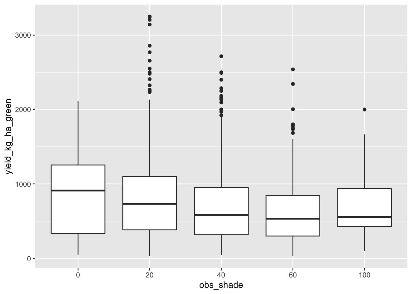
But there’s likely confounders here. Higher altitude farms might both get less shade and have soils less amenable to high yields.
data |> ggplot(aes(scale(farm_altitude_meters), log(yield_kg_ha_green))) + geom_point() + facet_wrap(~obs_shade) + geom_smooth()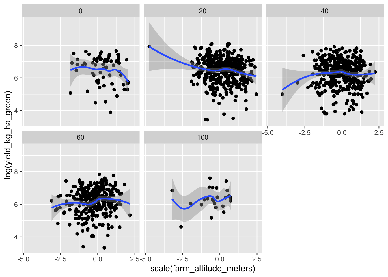
Let’s try modeling this more carefully.
fit <- lmer(log(yield_kg_ha_green) ~ obs_shade + (1|region/supply_unit) + scale(farm_altitude_meters), data=data)
tdat <- tibble(resid=residuals(fit))
tdat |> ggplot(aes(resid)) + geom_histogram()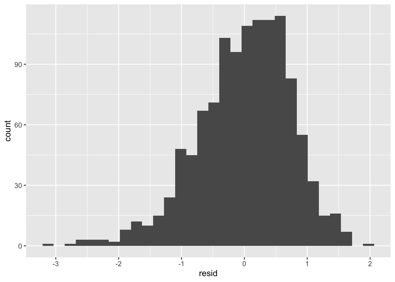
A log linear model seems a little skewed.
ggplot(tdat,aes(sample=resid)) + stat_qq() + stat_qq_line()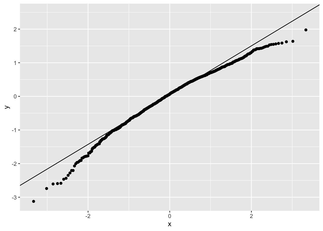
A GLM with a Gamma family works better here.
fit2 <- glmer(yield_kg_ha_green ~ obs_shade + scale(farm_altitude_meters) + (1|region/supply_unit), data=data, family=Gamma(link="log"))
plot(fit2)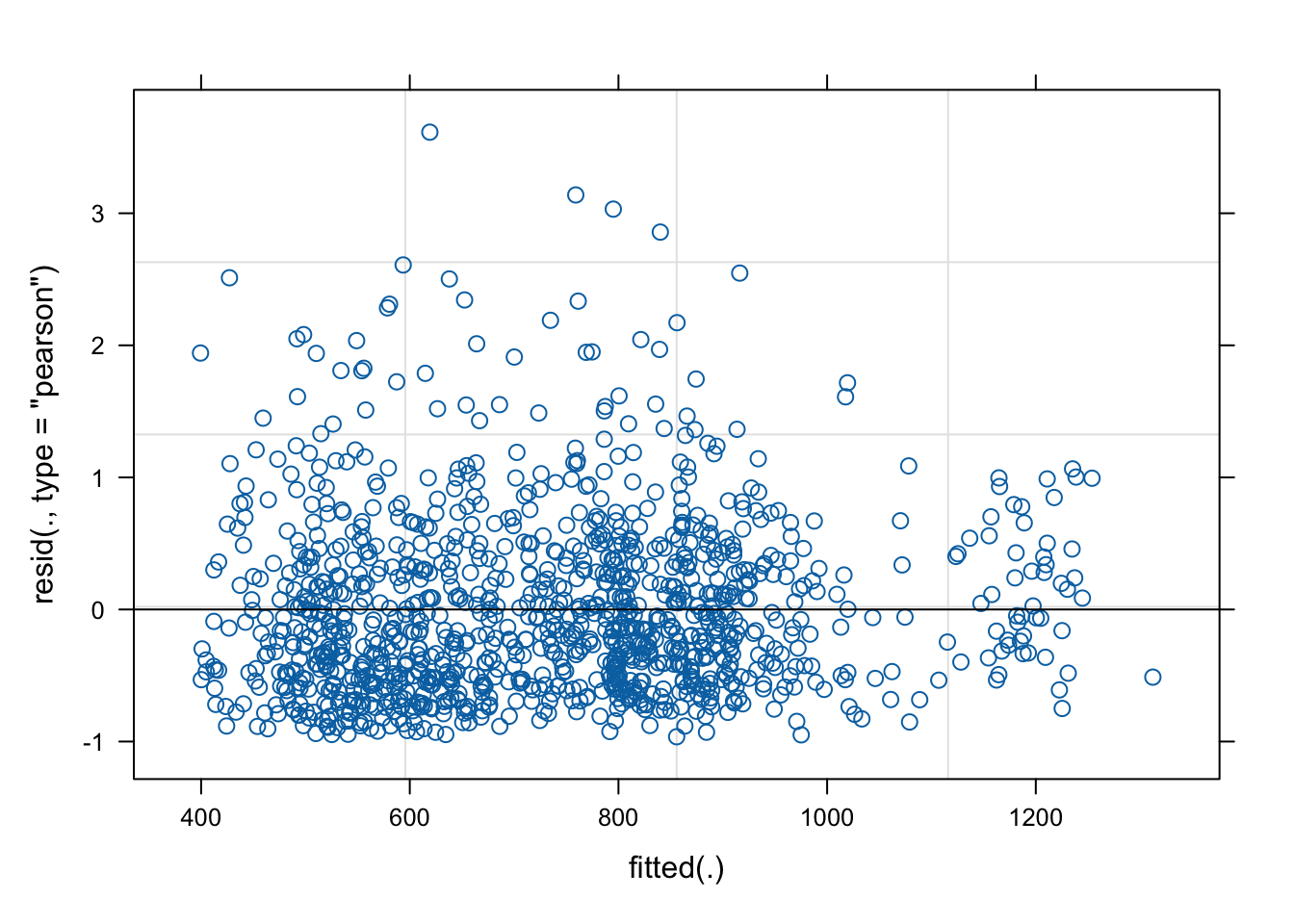
tibble(resid=residuals(fit2)) |> ggplot(aes(sample=resid)) + stat_qq() + stat_qq_line()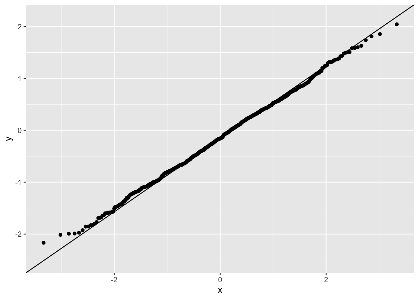
summary(fit2)Generalized linear mixed model fit by maximum likelihood (Laplace
Approximation) [glmerMod]
Family: Gamma ( log )
Formula: yield_kg_ha_green ~ obs_shade + scale(farm_altitude_meters) +
(1 | region/supply_unit)
Data: data
AIC BIC logLik -2*log(L) df.resid
17386.2 17431.8 -8684.1 17368.2 1159
Scaled residuals:
Min 1Q Median 3Q Max
-1.4288 -0.7563 -0.2222 0.5141 5.3585
Random effects:
Groups Name Variance Std.Dev.
supply_unit:region (Intercept) 0.05902 0.2429
region (Intercept) 0.03234 0.1798
Number of obs: 1168, groups: supply_unit:region, 20; region, 8
Fixed effects:
Estimate Std. Error t value Pr(>|z|)
(Intercept) 6.485595 0.092594 70.043 <2e-16 ***
obs_shade.L -0.233903 0.106634 -2.194 0.0283 *
obs_shade.Q 0.020627 0.088580 0.233 0.8159
obs_shade.C 0.045673 0.059994 0.761 0.4465
obs_shade^4 0.009596 0.039745 0.241 0.8092
scale(farm_altitude_meters) -0.037419 0.022113 -1.692 0.0906 .
---
Signif. codes: 0 '***' 0.001 '**' 0.01 '*' 0.05 '.' 0.1 ' ' 1
Correlation of Fixed Effects:
(Intr) obs_.L obs_.Q obs_.C obs_^4
obs_shade.L 0.135
obs_shade.Q 0.289 0.415
obs_shade.C 0.122 0.692 0.362
obs_shade^4 0.143 0.162 0.403 0.230
scl(frm_l_) 0.002 0.146 -0.033 0.028 0.019We see a pretty clear negative linear relationship between shade coverage and yield. To decrease the variance of our estimate, we can try controlling for other factors. Let’s factor in fertilizer use.
data |> ggplot(aes(scale(average_fertilizer_per_hectare), log(yield_kg_ha_green))) + geom_point() + geom_smooth(span=0.2)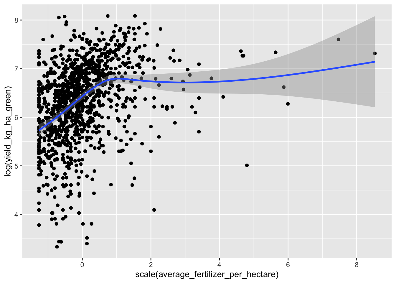
It seems like fertilizer has a highly nonlinear relationship with yield. Let’s just look at quantiles.
data <- data |> mutate(fertilizer_quantile = ntile(average_fertilizer_per_hectare, 4))data |> ggplot(aes(fertilizer_quantile, log(yield_kg_ha_green))) + geom_bar(stat="identity")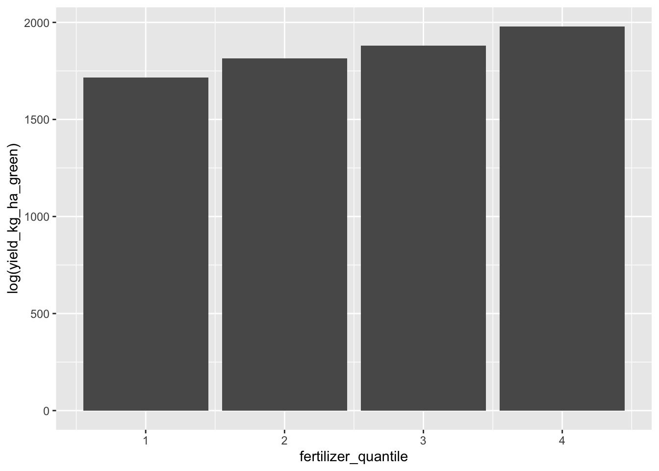
fit3 <- glmer(yield_kg_ha_green ~ obs_shade + scale(farm_altitude_meters) + fertilizer_quantile + (1|region/supply_unit), data=data, family=Gamma(link="log"))
summary(fit3)
Generalized linear mixed model fit by maximum likelihood (Laplace
Approximation) [glmerMod]
Family: Gamma ( log )
Formula: yield_kg_ha_green ~ obs_shade + scale(farm_altitude_meters) +
fertilizer_quantile + (1 | region/supply_unit)
Data: data
AIC BIC logLik -2*log(L) df.resid
17220.0 17270.6 -8600.0 17200.0 1158
Scaled residuals:
Min 1Q Median 3Q Max
-1.4805 -0.6998 -0.1895 0.4592 6.5325
Random effects:
Groups Name Variance Std.Dev.
supply_unit:region (Intercept) 0.05688 0.2385
region (Intercept) 0.01657 0.1287
Number of obs: 1168, groups: supply_unit:region, 20; region, 8
Fixed effects:
Estimate Std. Error t value Pr(>|z|)
(Intercept) 5.886119 0.088345 66.627 <2e-16 ***
obs_shade.L -0.248051 0.099910 -2.483 0.0130 *
obs_shade.Q 0.001488 0.083406 0.018 0.9858
obs_shade.C 0.015202 0.056538 0.269 0.7880
obs_shade^4 0.022442 0.037406 0.600 0.5485
scale(farm_altitude_meters) -0.034823 0.020595 -1.691 0.0909 .
fertilizer_quantile 0.233742 0.017419 13.418 <2e-16 ***
---
Signif. codes: 0 '***' 0.001 '**' 0.01 '*' 0.05 '.' 0.1 ' ' 1
Correlation of Fixed Effects:
(Intr) obs_.L obs_.Q obs_.C obs_^4 sc(__)
obs_shade.L 0.136
obs_shade.Q 0.293 0.414
obs_shade.C 0.140 0.691 0.364
obs_shade^4 0.127 0.161 0.402 0.227
scl(frm_l_) -0.010 0.151 -0.043 0.013 0.019
frtlzr_qntl -0.483 -0.008 -0.020 -0.039 0.027 0.010The AIC and residual variance decreased, and the standard error for shade’s negative linear effect shrunk even smaller.
plot(fit3)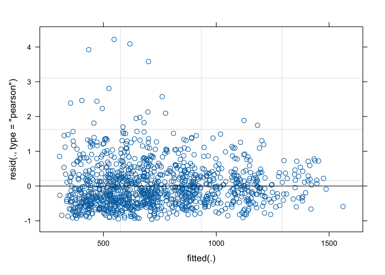
Finally, we can add in factors for the pest control efforts we extracted initially.
fit4 <- glmer(yield_kg_ha_green ~ obs_shade + scale(farm_altitude_meters) + fertilizer_quantile + use_insect_traps + biological_control + (1|region/supply_unit), data=data, family=Gamma(link="log"))
summary(fit4)
Generalized linear mixed model fit by maximum likelihood (Laplace
Approximation) [glmerMod]
Family: Gamma ( log )
Formula: yield_kg_ha_green ~ obs_shade + scale(farm_altitude_meters) +
fertilizer_quantile + use_insect_traps + biological_control +
(1 | region/supply_unit)
Data: data
AIC BIC logLik -2*log(L) df.resid
17217.0 17277.8 -8596.5 17193.0 1156
Scaled residuals:
Min 1Q Median 3Q Max
-1.4889 -0.6999 -0.1899 0.4686 6.6756
Random effects:
Groups Name Variance Std.Dev.
supply_unit:region (Intercept) 0.05524 0.2350
region (Intercept) 0.01718 0.1311
Number of obs: 1168, groups: supply_unit:region, 20; region, 8
Fixed effects:
Estimate Std. Error t value Pr(>|z|)
(Intercept) 5.87748 0.08827 66.586 <2e-16 ***
obs_shade.L -0.25083 0.09969 -2.516 0.0119 *
obs_shade.Q 0.00545 0.08338 0.065 0.9479
obs_shade.C 0.02022 0.05647 0.358 0.7203
obs_shade^4 0.02129 0.03738 0.570 0.5689
scale(farm_altitude_meters) -0.03168 0.02057 -1.540 0.1236
fertilizer_quantile 0.23140 0.01745 13.261 <2e-16 ***
use_insect_traps 0.18656 0.09333 1.999 0.0456 *
biological_control 0.12198 0.08625 1.414 0.1573
---
Signif. codes: 0 '***' 0.001 '**' 0.01 '*' 0.05 '.' 0.1 ' ' 1
Correlation of Fixed Effects:
(Intr) obs_.L obs_.Q obs_.C obs_^4 sc(__) frtlz_ us_ns_
obs_shade.L 0.135
obs_shade.Q 0.294 0.414
obs_shade.C 0.140 0.690 0.365
obs_shade^4 0.128 0.163 0.404 0.228
scl(frm_l_) -0.012 0.151 -0.041 0.015 0.020
frtlzr_qntl -0.476 -0.003 -0.016 -0.039 0.032 0.006
us_nsct_trp -0.012 0.012 0.053 0.045 0.027 0.040 0.003
blgcl_cntrl -0.039 -0.033 -0.045 -0.009 -0.052 0.035 -0.084 -0.099Interestingly, controlling for pest mitigation methods makes the effect of altitude seem much less significant. An analysis of deviance lets us compare the nested models.
anova(fit2, fit3, fit4)Data: data
Models:
fit2: yield_kg_ha_green ~ obs_shade + scale(farm_altitude_meters) + (1 | region/supply_unit)
fit3: yield_kg_ha_green ~ obs_shade + scale(farm_altitude_meters) + fertilizer_quantile + (1 | region/supply_unit)
fit4: yield_kg_ha_green ~ obs_shade + scale(farm_altitude_meters) + fertilizer_quantile + use_insect_traps + biological_control + (1 | region/supply_unit)
npar AIC BIC logLik -2*log(L) Chisq Df Pr(>Chisq)
fit2 9 17386 17432 -8684.1 17368
fit3 10 17220 17271 -8600.0 17200 168.2306 1 <2e-16 ***
fit4 12 17217 17278 -8596.5 17193 6.9538 2 0.0309 *
---
Signif. codes: 0 '***' 0.001 '**' 0.01 '*' 0.05 '.' 0.1 ' ' 1The difference in deviances (likelihood ratio) for model 4 is still significant.