using LinearAlgebra, StatsBase, StatsModels, LogExpFunctions, Random, Distributions, CairoMakie
CairoMakie.enable_only_mime!("png")
Say you want to fit a multivariate Normal distribution to some data.
Random.seed!(0)
Σ = rand(LKJ(3, 1))
μ = rand(3)
X = (μ .+ sqrt(Σ) * randn(3, 300))';
The obvious way to do this is with maximum likelihood estimation. In natural parameter form, the log likelihood is given by
\[ \sum_i x_i^T \Lambda \mu - \frac{1}{2} \text{Tr}(\Lambda x_i x_i^T) - N A(\eta) \] Derive wrt the natural parameters \(\eta = (\Lambda, \Lambda \mu)\) to get
\[ \begin{align*} \frac{1}{N}\sum_i x_i &= E[x] \frac{1}{N}\sum_i x_i x_i^T &= E[xx^T] \end{align*} \]
Easy. But now, how might you do this if some subset of the data is missing? We’ll assume that the data isn’t missing completely at random, so that our observed marginals aren’t unbiased estimators of the true marginals.
begin
missing_mask = rand(size(X, 1)) .< logistic.(-1 .+ X * -rand(size(X, 2), 3))
Xm = convert(Matrix{Union{Float64, Missing}}, X)
Xm[missing_mask] .= missing
sum(ismissing.(Xm); dims=1) ./ size(Xm, 1)
end
1×3 Matrix{Float64}:
0.25 0.263333 0.24We’re trying to find a maximum likelihood estimate in the presence of latent variables (in this case, all the unobserved values). It’s a classic situation for the EM algorithm!
At each step of EM, we want to find parameters \(\mu, \Sigma\) that maximize the expected log likelihood, where the expectation is taken with respect to \(p(x_\text{unobserved} | x_\text{observed})\). That’s
\[ \begin{align*} E\left[\sum_i x_i^T \Lambda \mu - \frac{1}{2} \text{Tr}(\Lambda x_i x_i^T) - N A(\eta)\right] = \sum_i E[x_i]^T \Lambda \mu - \frac{1}{2} \text{Tr}(\Lambda E[x_i x_i^T]) - N A(\eta) \end{align*} \]
Take the gradient as before to get
\[ \begin{align*} \mu &= \frac{1}{N}\sum_i E[y_i] \Sigma &= \frac{1}{N}\sum_i E[y_i y_i^T] \end{align*} \]
It remains to find out what \(E[x_i]\) and \(E[x_i x_i^T]\) are. For the components of \(x_i\) that are observed (call this subvector \(x_o\)), \(E[x_o] = x_o\). For the components \(x_u\) that are not observed, the Gaussian conditioning formula gives \(x_u = μ_u + Σ_{uo} Σ_{oo}^{-1}(y_o - μ_o)\)
function E_m1(x, μ, Σ)
    x2 = copy(x)
    u = ismissing.(x)
    o = .!u
    x2[u] .= μ[u] + Σ[u, o] * (Σ[o, o] \ (x[o] - μ[o]))
    x2
end;
The second moment breaks down similarly. \(E[x_i x_i^T]\) can be thought of (up to permutation) as a block matrix:
\[ \begin{bmatrix} x_o x_o^T & x_o x_u^T x_u x_o^T & x_u x_u^T \end{bmatrix} \]
As \(x_0\) and \(x_o x_o^T\) are known, that just leaves \(E[x_o x_u^T] = x_o \mu_u^T\) and \(E[x_u x_u^T] = \text{Var}(x_u | x_o) + \mu_u \mu_u^T\). The formula for conditional Gaussians tell us \(\text{Var}(x_u) = \Sigma_{uu} - \Sigma_{uo} \Sigma_{oo}^{-1} \Sigma_{ou}\).
function E_m2(x, μ, Σ)
    x2 = Matrix{Float64}(undef, size(Σ))
    u = ismissing.(x)
    o = .!u
    x2[o,o] .= x[o] * x[o]'
    x2[o, u] .= x[o] * μ[u]'
    x2[u, o] .= x2[o, u]'
    x2[u,u] = Σ[u,u] - Σ[u, o] * (Σ[o,o] \ Σ[o, u]) + μ[u]*μ[u]'
    x2
end;
Let’s put it all together!
function em_step(X, μ, Σ)
μ = mean(E_m1(x, μ, Σ) for x in eachrow(X))
m2 = mean(E_m2(x, μ, Σ) for x in eachrow(X))
(μ, m2 - μ * μ')
end
function em_alg(X, μ, Σ)
for _ in 1:100
μ2, Σ2 = em_step(X, μ, Σ)
δ = max(maximum(abs.(μ - μ2)), maximum(abs.(Σ2 - Σ)))
if δ < 1e-5
return (μ, Σ)
end
μ, Σ = (μ2, Σ2)
end
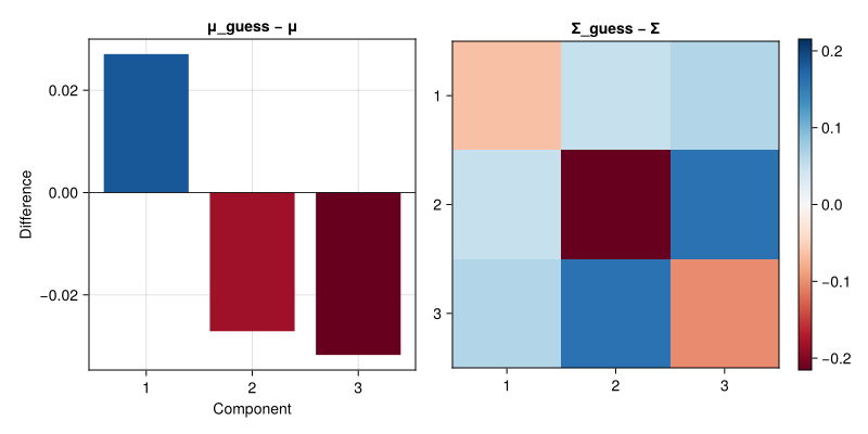
end;μ_guess, Σ_guess = em_alg(Xm, randn(3), 1.0I(3));Our guess is pretty close to the true value!
let
    diff_μ = μ_guess - μ
    diff_Σ = Σ_guess - Σ

    fig = Figure(size=(800, 400))

    # Vector difference: bar chart
    ax1 = Axis(fig[1, 1], title="μ_guess − μ", xlabel="Component", ylabel="Difference",
               xticks=(1:3, ["1", "2", "3"]))
    clim_μ = maximum(abs.(diff_μ))
    barplot!(ax1, 1:3, diff_μ,
             color=diff_μ, colormap=:RdBu, colorrange=(-clim_μ, clim_μ))
    hlines!(ax1, [0], color=:black, linewidth=0.8)

    # Matrix difference: heatmap
    clim_Σ = maximum(abs.(diff_Σ))
    ax2 = Axis(fig[1, 2], title="Σ_guess − Σ", aspect=DataAspect(),
               yreversed=true,
               xticks=(1:3, ["1", "2", "3"]),
               yticks=(1:3, ["1", "2", "3"]))
    hm = heatmap!(ax2, diff_Σ, colormap=:RdBu, colorrange=(-clim_Σ, clim_Σ))
    Colorbar(fig[1, 3], hm)

    fig
end