This tutorial demonstrates how to perform audio source separation using the SepReformer architecture. We’ll use equinoix for the neural network, with beartype for runtime type checking.
import numpy as np
import jax
import jax.numpy as jnp
import equinox as eqx
from jaxtyping import Float, Array, jaxtyped
from beartype import beartype
import soundfile as sf
The Task
Given a mono mixture waveform \(x \in \mathbb{R}^T\), produce \(N\) separated stem waveforms \(\hat{s}_1, \ldots, \hat{s}_N \in \mathbb{R}^T\) such that \(\sum_n \hat{s}_n \approx x\) and each \(\hat{s}_n\) matches one isolated voice track.
We use the JaCappella corpus (35 a cappella songs) via Hugging Face. Each song has 5 isolated stems — lead_vocal, soprano, alto, tenor, bass — and the mixture is their sum.
import librosa
from pathlib import Path

STEM_NAMES = ("lead_vocal", "soprano", "alto", "tenor", "bass")
SAMPLE_RATE = 44100

class JaCappellaDataset:
    def __init__(self, root) -> None:
        self.root = Path(root)
        self.sample_rate = 44100
        self.songs = sorted(
            song
            for genre in self.root.iterdir()
            if genre.is_dir() and not genre.name.startswith(".")
            for song in genre.iterdir()
            if song.is_dir() and not song.name.startswith("."))

    @jaxtyped(typechecker=beartype)
    def _load_wav(self, path: Path) -> Float[np.ndarray, "T"]:
        """Load a wav file, resample if needed, return mono float32."""
        audio, sr = sf.read(path, dtype="float32", always_2d=True)
        audio = audio[:, 0]  # take first channel if stereo
        if sr != self.sample_rate:
            audio = librosa.resample(audio, orig_sr=sr, target_sr=self.sample_rate)
        return audio

    @jaxtyped(typechecker=beartype)
    def _load_stems(self, song_dir: Path) -> Float[np.ndarray, "N T"]:
        """Load all available stems for a song."""
        stems = []
        for i, name in enumerate(STEM_NAMES):
            path = song_dir / f"{name}.wav"
            stems.append(self._load_wav(path) if path.exists() else np.zeros(0, dtype=np.float32))
        max_len = max(len(s) for s in stems)
        result = np.zeros((5, max_len), dtype=np.float32)
        for i, s in enumerate(stems):
            result[i, :len(s)] = s
        return result

    @jaxtyped(typechecker=beartype)
    def __getitem__(self, idx: int) -> tuple[Float[np.ndarray, "T"], Float[np.ndarray, "N T"]]:
        """Load full song."""
        song_dir = self.songs[idx]
        stems = self._load_stems(song_dir)
        return stems.sum(axis=0), stems

    def __len__(self) -> int:
        return len(self.songs)

dataset = JaCappellaDataset("/space/samanklesaria/data/jacappella")
We’ll feed the dataset to our model using the grain library.
import grain

SEG_SAMPLES = SAMPLE_RATE * 2   # 2-second segments
BATCH_SIZE  = 1

def extract_segment(item, rng):
    mixture, stems = item
    T = mixture.shape[0]
    if T <= SEG_SAMPLES:
        pad = SEG_SAMPLES - T
        return np.pad(mixture, (0, pad)), np.pad(stems, ((0, 0), (0, pad)))
    start = rng.integers(0, T - SEG_SAMPLES)
    return mixture[start:start + SEG_SAMPLES], stems[:, start:start + SEG_SAMPLES]

def batch_to_jax(items):
    mixtures = jnp.array(np.stack([m for m, _ in items]))  # (B, T)
    stems    = jnp.array(np.stack([s for _, s in items]))  # (B, N, T)
    return mixtures, stems

loader = (grain.MapDataset.source(dataset)
        .seed(0).shuffle()
        .random_map(extract_segment)
        .batch(BATCH_SIZE, drop_remainder=True, batch_fn=batch_to_jax))
To make sure the data is loading correctly, we can sample a batch and log it to Tensorboard.
from tensorboardX import SummaryWriter

mixture, stems = next(iter(loader))
mixture = np.array(mixture[0])  # (T,)
stems = np.array(stems[0])      # (N, T)
writer = SummaryWriter("samples")
peak = np.max(np.abs(mixture))
scale = 0.99 / peak if peak > 0 else 1.0
writer.add_audio(
    f"mixture",
    mixture * scale,
    sample_rate=dataset.sample_rate)
for n in range(stems.shape[0]):
    writer.add_audio(
        f"stem/{n}",
        stems[n] * scale,
        sample_rate=dataset.sample_rate)
writer.close()Architecture
At a high level: - The input waveform is encoded to a latent space using convolutional and transformer layers. - The result gets split into separate pieces for each voice part - Each piece is decoded back to a waveform by the same stack of transformer and convolutional layers.
\[x \xrightarrow{\text{Conv}} h \xrightarrow{\text{Enc blocks}} h \xrightarrow{\text{Split}} \{h_n\} \xrightarrow{\text{Dec blocks (vmapped)}} \xrightarrow{\text{ConvT (vmapped)}} \{\hat{s}_n\}\]
Convolutional Layers: Waveform → Latent Frames and Back
A strided 1-D convolution converts the raw waveform into a sequence of latent frames. With kernel \(K\) and stride \(S\):
\[L = \left\lfloor \frac{T - K}{S} \right\rfloor + 1\]
The encoder applies a GELU after the convolution:
\[h = \text{GELU}(W_\text{enc} * x), \quad h \in \mathbb{R}^{L \times C}\]
class Encoder(eqx.Module):
    conv: eqx.nn.Conv1d

    def __init__(self, out_channels: int, key: jax.random.PRNGKey):
        self.conv = eqx.nn.Conv1d(1, out_channels, 16, stride=8, key=key)

    def __call__(self, x: Float[Array, "T"]) -> Float[Array, "L C"]:
        h = self.conv(x[None, :])   # (C, L)
        h = jax.nn.gelu(h)
        return jnp.transpose(h)     # (L, C)
class Decoder(eqx.Module):
conv_t: eqx.nn.ConvTranspose1d
def __init__(self, in_channels, key: jax.random.PRNGKey):
self.conv_t = eqx.nn.ConvTranspose1d(in_channels, 1, 16, stride=8, key=key)
@jaxtyped(typechecker=beartype)
def __call__(self, h: Float[Array, "L C"]) -> Float[Array, "T"]:
h = jnp.transpose(h) # (C, L)
out = self.conv_t(h) # (1, T)
return out[0] # (T,)Default: \(K=16\), \(S=8\), \(C=256\). At 44.1 kHz a 2-second clip becomes \(L \approx 11{,}025\) frames.
SNAKE Activation
SNAKE (Liu et al., 2022) adds a learnable sinusoidal term that preserves the periodic structure present in harmonic audio:
\[\text{SNAKE}(x; \alpha) = x + \frac{1}{\alpha}\sin^2(\alpha x)\]
\(\alpha\) is initialized to \(\mathbf{1}\) (small perturbation at startup) and learned per channel. SNAKE is used inside every feed-forward sub-layer in the transformer blocks.
class Snake(eqx.Module):
    alpha: Array   # (F,), one per feature

    def __init__(self, features: int, *, key: jax.random.PRNGKey):
        self.alpha = jnp.ones(features)

    def __call__(self, x: Float[Array, "... F"], **_) -> Float[Array, "... F"]:
        return x + (1.0 / (self.alpha + 1e-6)) * jnp.sin(self.alpha * x) ** 2
def feedforward(dim, ff_dim, key: jax.random.PRNGKey):
k1, k2, k3 = jax.random.split(key, 3)
return eqx.nn.Sequential([
eqx.nn.Linear(dim, ff_dim, key=k1),
Snake(ff_dim, key=k2),
eqx.nn.Linear(ff_dim, dim, key=k3)])class TransformerBlock(eqx.Module):
norm1: eqx.nn.LayerNorm
norm2: eqx.nn.LayerNorm
attn: eqx.nn.MultiheadAttention
ff: eqx.nn.Sequential
rope: eqx.nn.RotaryPositionalEmbedding
scale1: Array
scale2: Array
def __init__(
self, dim: int, num_heads: int, ff_dim: int, *, key: jax.random.PRNGKey
):
k1, k2 = jax.random.split(key)
self.norm1 = eqx.nn.LayerNorm(dim)
self.attn = eqx.nn.MultiheadAttention(
num_heads=num_heads, query_size=dim, key=k1
)
self.norm2 = eqx.nn.LayerNorm(dim)
self.ff = feedforward(dim, ff_dim, key=k2)
self.rope = eqx.nn.RotaryPositionalEmbedding(dim // num_heads)
self.scale1 = jnp.full(dim, 1e-4)
self.scale2 = jnp.full(dim, 1e-4)
@jaxtyped(typechecker=beartype)
def __call__(self, x: Float[Array, "S D"]) -> Float[Array, "S D"]:
normed = jax.vmap(self.norm1)(x)
def process_heads(q, k, v):
q = jax.vmap(self.rope, in_axes=1, out_axes=1)(q)
k = jax.vmap(self.rope, in_axes=1, out_axes=1)(k)
return q, k, v
attn_out = self.attn(normed, normed, normed, process_heads=process_heads)
x = x + self.scale1 * attn_out
x = x + self.scale2 * jax.vmap(self.ff)(jax.vmap(self.norm2)(x))
return xStacking Transformer Layers: The Dual-Path Approach
Full self-attention over \(L \approx 11{,}000\) frames costs \(O(L^2)\). The dual-path trick (Luo & Mesgarani, 2020) splits this into two \(O(L \cdot K)\) passes:
- Intra-chunk — reshape to \((M, K, C)\); each of the \(M\) chunks attends within itself. Captures local patterns. Cost: \(O(M \cdot K^2)\).
- Inter-chunk — transpose to \((K, M, C)\); each time-slot attends across all \(M\) chunks. Propagates global pitch/rhythm. Cost: \(O(K \cdot M^2)\).
class DualPathBlock(eqx.Module):
    intra_block: TransformerBlock
    inter_block: TransformerBlock
    chunk_size: int = eqx.field(static=True)

    def __init__(
        self,
        dim: int,
        num_heads: int,
        ff_dim: int,
        chunk_size: int = 64,
        *,
        key: jax.random.PRNGKey,
    ):
        k1, k2 = jax.random.split(key)
        self.intra_block = TransformerBlock(dim, num_heads, ff_dim, key=k1)
        self.inter_block = TransformerBlock(dim, num_heads, ff_dim, key=k2)
        self.chunk_size = chunk_size

    @jaxtyped(typechecker=beartype)
    def __call__(self, x: Float[Array, "L C"]) -> Float[Array, "L C"]:
        L, C = x.shape
        K = self.chunk_size

        # Pad to multiple of chunk_size
        pad_len = (K - L % K) % K
        if pad_len > 0:
            x = jnp.pad(x, ((0, pad_len), (0, 0)))

        L_padded = x.shape[0]
        num_chunks = L_padded // K

        # Reshape to (num_chunks, chunk_size, C)
        chunks = x.reshape(num_chunks, K, C)

        # Intra-chunk attention: attend within each chunk
        chunks = jax.vmap(self.intra_block)(chunks)  # (num_chunks, K, C)

        # Inter-chunk attention: transpose to (K, num_chunks, C), attend across chunks
        inter = jnp.transpose(chunks, (1, 0, 2))  # (K, num_chunks, C)
        inter = jax.vmap(self.inter_block)(inter)  # (K, num_chunks, C)
        chunks = jnp.transpose(inter, (1, 0, 2))  # (num_chunks, K, C)

        # Reshape back
        out = chunks.reshape(L_padded, C)
        return out[:L]  # remove padding
Splitting into Speaker Streams
After the shared encoder blocks, a SplitLayer expands \((L, C)\) into \((N,
L, C)\). Splitting here lets each of the \(N\) reconstruction stacks specialize on one speaker while sharing parameters (via vmap) to keep the model compact.
A GLU gate first refines the shared features before expanding:
\[g, v = \text{split}(W_1 h), \quad h' = \sigma(g) \odot v, \quad \text{streams} = W_2 h' \;\text{reshaped to}\; (N, L, C)\]
class SplitLayer(eqx.Module):
    linear1: eqx.nn.Linear  # C → 2C
    linear2: eqx.nn.Linear  # C → N*C
    num_stems: int

    def __init__(self, dim: int, num_stems: int, *, key: jax.random.PRNGKey):
        k1, k2 = jax.random.split(key)
        self.linear1 = eqx.nn.Linear(dim, dim * 2, key=k1)
        self.linear2 = eqx.nn.Linear(dim, dim * num_stems, key=k2)
        self.num_stems = num_stems

    def __call__(self, x: Float[Array, "L C"]) -> Float[Array, "N L C"]:
        h = jax.vmap(self.linear1)(x)               # (L, 2C)
        gate, val = jnp.split(h, 2, axis=-1)
        h = jax.nn.sigmoid(gate) * val              # (L, C)
        h = jax.vmap(self.linear2)(h)               # (L, N*C)
        h = h.reshape(x.shape[0], self.num_stems, -1)
        return jnp.transpose(h, (1, 0, 2))          # (N, L, C)
Full Forward Pass
With all the building blocks in place, we can now assemble the complete SepReformer model. The forward pass threads the input waveform through the encoder, a stack of dual-path separation blocks, the split layer, a stack of dual-path reconstruction blocks (applied independently to each stem via vmap), and finally the decoder (also vmapped across stems). The output is trimmed or padded to match the original waveform length.
class SepReformer(eqx.Module):
    encoder: Encoder
    sep_blocks: list[DualPathBlock]
    split: SplitLayer
    rec_blocks: list[DualPathBlock]
    decoder: Decoder

    def __init__(self, key: jax.random.PRNGKey):
        num_sep_blocks = 2
        num_rec_blocks = 2
        dim = 256
        num_heads = 8
        ff_dim = 1024
        chunk_size = 64

        num_blocks = num_sep_blocks + num_rec_blocks
        keys = jax.random.split(key, 3 + num_blocks)
        self.encoder = Encoder(dim, keys[0])
        self.decoder = Decoder(dim, keys[1])
        self.split = SplitLayer(dim, 5, key=keys[2])
        self.sep_blocks = [
            DualPathBlock(dim, num_heads, ff_dim, chunk_size, key=keys[3 + i])
            for i in range(num_sep_blocks)
        ]
        self.rec_blocks = [
            DualPathBlock(dim, num_heads, ff_dim, chunk_size, key=keys[3 + num_sep_blocks + i])
            for i in range(num_rec_blocks)
        ]


    def __call__(self, x: Float[Array, "T"]) -> Float[Array, "N T"]:
        h = self.encoder(x)
        for block in self.sep_blocks:
            h = block(h)
        stems = self.split(h)                    # (N, L, C)
        for block in self.rec_blocks:
            stems = jax.vmap(block)(stems)
        out = jax.vmap(self.decoder)(stems)      # (N, T')
        # trim / pad to original length
        T = x.shape[0]
        if out.shape[1] > T:
            out = out[:, :T]
        elif out.shape[1] < T:
            out = jnp.pad(out, ((0, 0), (0, T - out.shape[1])))
        return out

model = SepReformer(jax.random.PRNGKey(0))
Loss Functions
Supervising a source separator is not straightforward. A plain mean-squared error (MSE) in the waveform domain penalises tiny timing offsets and global loudness differences equally, so the model spends capacity chasing irrelevant phase shifts rather than learning to separate voices. We instead use two complementary objectives — one waveform-domain and one spectral — that together give stable, perceptually meaningful gradients.
SI-SDR
SI-SDR projects the estimate onto the target and reports the energy ratio in dB. It is invariant to global loudness, which matters for a cappella where voices differ widely in level:
\[\hat{s}_\text{tgt} = \frac{\langle \hat{s}, s \rangle}{\|s\|^2} s, \qquad \text{SI-SDR} = 10\log_{10}\frac{\|\hat{s}_\text{tgt}\|^2}{\|\hat{s} - \hat{s}_\text{tgt}\|^2}\]
The projection step removes any DC offset before computing the ratio, so a perfectly separated signal that is merely scaled up or down still scores the maximum possible value. In practice, SI-SDR values above \(+10\ \text{dB}\) indicate clearly separated sources; below \(0\ \text{dB}\) the estimate is dominated by leakage from other voices. We negate it to turn maximisation into minimisation.
@jaxtyped(typechecker=beartype)
def si_sdr(estimate: Float[Array, "T"], target: Float[Array, "T"], eps: float = 1e-8) -> Float[Array, ""]:
    estimate = estimate - jnp.mean(estimate)
    target   = target   - jnp.mean(target)
    dot      = jnp.sum(estimate * target)
    s_target = (dot / (jnp.sum(target ** 2) + eps)) * target
    e_noise  = estimate - s_target
    return 10.0 * jnp.log10(jnp.sum(s_target ** 2) / (jnp.sum(e_noise ** 2) + eps) + eps)
Multi-Resolution STFT Loss
SI-SDR is blind to spectral texture: two signals can have the same SI-SDR yet sound very different if one has unnatural resonances or missing harmonics. Adding a frequency-domain term at three FFT scales \(\{512, 1024, 2048\}\) addresses this at multiple time-frequency resolutions simultaneously.
A small FFT (\(512\)) gives sharp time resolution — useful for detecting onset smearing — while a large FFT (\(2048\)) gives fine frequency resolution — useful for resolving individual harmonics in a choir. Using all three averages out the inherent time-frequency tradeoff of any single STFT.
Each scale contributes two terms:
- Spectral convergence — the Frobenius-norm distance between magnitude spectrograms, normalised by the target energy. This drives the gross shape of the spectrum towards the reference.
- Log-magnitude distance — the mean absolute difference on a log scale. Because human pitch perception is logarithmic, this term penalises errors in quiet harmonics just as strongly as errors in loud ones.
\[\mathcal{L}_\text{STFT} = \frac{1}{3}\sum_\text{scale}\left(\underbrace{\frac{\||S| - |\hat{S}|\|_F}{\||S|\|_F}}_{\text{spectral convergence}} + \underbrace{\text{mean}|\log|S| - \log|\hat{S}||}_{\text{log-magnitude}}\right)\]
@jaxtyped(typechecker=beartype)
def stft_mag(x: Float[Array, "T"], fft_size: int, hop: int, win_size: int) -> Float[Array, "F K"]:
    window = jnp.hanning(win_size)
    x_pad  = jnp.pad(x, (fft_size // 2, fft_size // 2))
    n_frames = (len(x_pad) - win_size) // hop + 1
    idx    = jnp.arange(win_size)[None, :] + jnp.arange(n_frames)[:, None] * hop
    frames = x_pad[idx] * window
    return jnp.abs(jnp.fft.rfft(frames, n=fft_size, axis=-1)).T  # (F, K)

@jaxtyped(typechecker=beartype)
def stft_loss_single(est: Float[Array, "T"], tgt: Float[Array, "T"], fft_size: int, hop: int, win: int) -> Float[Array, ""]:
    em, tm = stft_mag(est, fft_size, hop, win), stft_mag(tgt, fft_size, hop, win)
    sc = jnp.linalg.norm(tm - em) / (jnp.linalg.norm(tm) + 1e-8)
    lm = jnp.mean(jnp.abs(jnp.log(em + 1e-8) - jnp.log(tm + 1e-8)))
    return sc + lm

@jaxtyped(typechecker=beartype)
def mr_stft_loss(est: Float[Array, "T"], tgt: Float[Array, "T"]) -> Float[Array, ""]:
    scales = [(512, 128, 512), (1024, 256, 1024), (2048, 512, 2048)]
    return sum(stft_loss_single(est, tgt, *s) for s in scales) / len(scales)
Composite Loss
The final objective combines the two terms, with the STFT loss weighted at \(0.5\) so that SI-SDR — which operates directly in the waveform domain and carries the strongest perceptual signal — dominates early in training. The STFT term then fills in spectral detail that SI-SDR cannot see. Both terms are averaged across the \(N\) stems before being averaged across the batch.
@jaxtyped(typechecker=beartype)
def composite_loss(estimates: Float[Array, "N T"], targets: Float[Array, "N T"]) -> Float[Array, ""]:
    def pair(est, tgt):
        return -si_sdr(est, tgt) + 0.5 * mr_stft_loss(est, tgt)
    return jnp.mean(jax.vmap(pair)(estimates, targets))

@eqx.filter_value_and_grad
def loss_fn(m, mixture: Float[Array, "B T"], targets: Float[Array, "B N T"]) -> Float[Array, ""]:
    def single(mix, tgt):
        return composite_loss(m(mix), tgt)
    return jnp.mean(jax.vmap(single)(mixture, targets))
Overfitting on JaCappella
Before training on the full corpus, we overfit on a single batch. This is a fast sanity check: if the model cannot memorise even one example, something is wrong with the architecture, the loss, or the data pipeline. It is much cheaper to discover this now than after a multi-hour training run.
Audio Logging
The loss curve tells you the model is learning, but it does not tell you what it is learning. Listening to the actual estimates at checkpoints is irreplaceable: you can hear immediately whether the model is separating voices, producing silence, or emitting noise. log_audio_samples writes one batch of audio to TensorBoard — the raw mixture, each ground-truth stem, and the corresponding model estimate — all normalised to a peak of \(0.99\) so playback levels are comparable across steps.
def log_audio_samples(model, loader, writer, global_step):
    mixture, stems = next(iter(loader))
    mix_np = np.array(mixture[0])
    stems_np = np.array(stems[0])
    est_np = np.array(model(mixture[0]))
    scale  = 0.99 / (np.max(np.abs(mix_np)) + 1e-8)
    writer.add_audio("mixture", mix_np * scale, global_step, sample_rate=SAMPLE_RATE)
    for n in range(stems_np.shape[0]):
        writer.add_audio(f"true/{n}", stems_np[n] * scale, global_step, sample_rate=SAMPLE_RATE)
    for n in range(est_np.shape[0]):
        est_scale  = 0.99 / (np.max(np.abs(est_np[n])) + 1e-8)
        writer.add_audio(f"estimate/{n}", est_np[n] * est_scale, global_step, sample_rate=SAMPLE_RATE)
Optimizer and Training Loop
We use AdamW with a global gradient-norm clip of \(1.0\). Clipping is important here because early in training the split layer and decoder produce near-random outputs, which can generate very large gradients through the SI-SDR loss. Weight decay of \(10^{-2}\) provides mild regularisation to prevent any single stem stream from collapsing to zero.
While training, you can monitor progress in TensorBoard with tensorboard --logdir runs/overfit.
@eqx.filter_jit
def step(model, opt_state, mixture, targets):
    loss, grads = loss_fn(model, mixture, targets)
    updates, opt_state = optimizer.update(grads, opt_state, model)
    return eqx.apply_updates(model, updates), opt_state, loss
import optax
optimizer = optax.chain(optax.clip_by_global_norm(1.0), optax.adamw(3e-4, weight_decay=1e-2))
opt_state = optimizer.init(eqx.filter(model, eqx.is_array))
writer = SummaryWriter("runs/overfit")
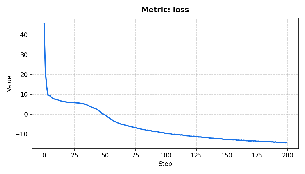
for epoch in range(200):
for mixture, targets in loader[:1]:
model, opt_state, loss = step(model, opt_state, mixture, targets)
writer.add_scalar("loss", float(loss), epoch)
if epoch % 20 == 0:
log_audio_samples(model, loader, writer, epoch)
writer.close()The exported Tensorboard results are shown below:
Scalar Trend: loss
|
Step Scrubber0
|
Step Scrubber0
|
Step Scrubber0
|
|
Step Scrubber0
|
Step Scrubber0
|