
Hop Lists
Introduction
Hop Lists are a novel retroactive set data-structure that allow for a branching timeline. Each hop list node $h_t$ is associated with a specific time $t$ and a randomly chosen height $L_t$. The interface consists of three methods:
- $\text{current}(h_t)$ gets the set of elements we would see at time $t$.
- $\text{advance}(h_t)$ creates a new node $h_{t+1}$ allowing queries about the set at time $t+1$.
- $\text{push}(h_t, v)$ pushes the value $v$ into the set at time $t$. This value will now appear in the sets associated with all future times $t’ >t$.
Hop lists nodes store four fields: a set of underlying type $S$, a pointer to a predecessor node with heigh at least $L_t$, a list of the most recent nodes at each height, and a list of pointers to specific future nodes.
@kwdef struct HopNode{S}
    "The new elements since `pred`."
    set::S = S()
    "The most recent node at the same height as this one or higher"
    pred::Union{Nothing,HopNode{S}} = nothing
    "(Node, height) pairs sorted by height giving the most recent node at that height"
    levels::LinkedList{Pair{HopNode{S}, Int}} = nil(Pair{HopNode{S}, Int})
    "Nodes to update when this node gets updated"
    succs::Vector{HopNode{S}} = HopNode{S}[]
end
Hop lists maintain the Predecessor Property: If hop node $h_t$ has predecessor $h_s$, then $h_t$’s set must store all the elements pushed at times in the interval $(s, t]$.
This means we can find $\text{current}(h_t)$ by taking the union of $h_t$’s ancestors.
# Iteration jumps back through `pred` edges
Base.iterate(h::HopNode, s::HopNode=h) = (s, s.pred)
Base.iterate(h::HopNode, ::Nothing) = nothing
Base.IteratorSize(::Type{HopNode{S}}) where {S} = Base.SizeUnknown()
Base.eltype(::Type{HopNode{S}}) where {S} = HopNode{S}

current(h::HopNode) = mapreduce(a -> a.set, union, h)
When we create a new hop node $h_{t’} = \text{advance}(h_t)$, we will set the predecessor to be h_t.levels[l] where $l = L_{t’} \sim \text{Geom}(0.5)$. To ensure that we maintain the predecessor property, we must take the the union of all the predecessor sets we find this way and store them in the new node’s set. The new levels list should remove all entries below $L_t$ and add $h_t$.
function advance(h::HopNode)
    n = 1 + rand(Geometric(0.5))
    pred = getpred(h.levels, n)
    itr = takewhile(x->x!=pred, h)
    result = HopNode(;pred, set=mapreduce(a->a.set, union, itr))
    result.levels = cons(result=>n, listdrop(h.levels, n))
    result
end
This uses the utility functions listdrop and getpred
function listdrop(l::LinkedList{Pair{A,Int}}, k::Int) where {A}
    while !isempty(l)
        (_,a) = l.head
        a > k && return l
        l = l.tail
    end
    l
end

function getpred(l::LinkedList{Pair{A,Int}}, n::Int) where {A}
    pred = nothing
    for (p, height) in l
        if height >= n
            pred = p
            break
        end
    end
    pred
end
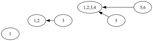
For example, if we inserted 1 at time 1, 2 at time 2, and so on up to 6, we might get a HopNode structure that looks like this The black arrows here correspond to pred pointers, the x axis corresponds to time, and the $y$ axis gives the height $L_t$ of each node $h_t$.
The tricky part is handling $\text{push}$. We need to give each node $h_s$ pointers to all future nodes $h_t$ for which h_s.set $\subseteq$ h_t.set That way, when we push into $h_s$, we know to push into $h_t$ as well. This list of pointers will be our succs vector. The idea results in the following code.
function Base.push!(t::HopNode{S}, v) where {S}
    q = HopNode{S}[t]
    while !isempty(q)
        t = pop!(q)
        push!(t.set, v)
        append!(q, t.succs)
    end
end
We still need to create these succs pointers in the first place. Each node should have an element of succs pointing to the closest future node with a higher height if one exists.
To fit these requirements, we can modify the advance method as follows:
function advance(h::HopNode)
    n = 1 + rand(Geometric(0.5))
    pred = getpred(h.levels, n)
    itr = takewhile(x->x!=pred, h)
    result = HopNode(set=mapreduce(a->a.set, union, itr))
    for t in itr
        push!(t.succs, result)
    end
    result.levels = cons(result=>n, listdrop(h.levels, n))
    result
end
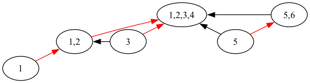
With the succs pointers visualized in red, the previous example looks as follows:
Note that advance can be called twice on the same node $h_t$, producing a branching timeline. Updates to $h_t$ will be propagated to both possible futures. This is why we need succs to be a vector rather than simply an optional pointer.
Average Time and Space Complexity
If the size of our timeline is $n$, we’ll have on average $n$ nodes with height $\geq 1$, $n/2$ nodes with height $\geq 2$, and so on up to $1$ node with height $\log n$. If we perform a current query from a node at height $1$, it takes on average $2$ hops through predecessor nodes to get to a node with height $\geq 2$. This means that after at most $2 \log n$ hops on average we should be at the node with height $\log n$ which has no predecessors. Therefore, the average number of sets we must union to answer a current query is $O(\log n)$ in expectation.
The average time complexity for push can be found analogously. The push operation follows succ pointers, where the successor to a node is the closest future node with a higher height, if one exists. As traversing each succ pointer takes us to a higher height, the time complexity of push is just the largest height of any node in our timeline, which on average is also $O(\log n)$.
The same logic allows us to find space complexity. Say we store at most $c$ elements in each time-slot. We know that the set associated with any time $t$ will be replicated at most $\log n$ times. So we use at most $cn \log n = O(n \log n)$ space for the set fields. For the levels field, each HopNode creates a single linked list node for its levels list, so this contributes $O(n)$ space. Each node’s succs field will contain at most one element if the timeline does not branch, so once again we get a linear space contribution. This gives total space complexity $O(n \log n)$.
Concentration Bounds
We know from the previous section that the time it takes to insert an element is at most the maximum height of any node in the timeline. The probability that the maximum height of any node in a timeline is above $k$ is \(\begin{align*} &1 - \prod_{i=1}^n P(h_i \text{ has height below $k$}) \\ &= 1 - (1 - 2^{-k})^n \end{align*}\) For $k=2\log_2 n$, we get \(1 - \left(1 - \frac{1}{n^2}\right)^n\) But $\lim_{n \to \infty} \left(1 - \frac{1}{n^2}\right)^n = 1$. So the probability of insertion being any worse than $2\log_2 n$ goes to zero.
To bound the number of backward hops taken by current queries, we can find the probability it takes $\leq k$ hops to iterate backwards from a node $h_n$ with height $1$. We can lower bound this by the probability that it takes $\leq k/L$ hops to get to a node with height 2, times the probability it takes $\leq k/L$ hops to get to a node with height 3, and so on up to the maximum height $L$. This is
\((1 - 2^{-k/L})^L\)
For $k = 2L\log_2 L$, we get the probability
\(\left(1 - \frac{1}{L^2}\right)^L\)
As $L \to \infty$ this converges to $1$, meaning that the probability a current query takes more than $2 L \log_2L$ time falls to zero.
Height-Free Variant
We can construct a variant of the data structure described that does not use a levels list. Instead, when we create a new hop node $h_{t’} = \text{advance}(h_t)$, we will set the predecessor by sampling $n \sim \text{Geom}(0.5)$ and then taking $n$ predecessor hops back from $h_t$. Specifically, we would have
function advance(t::HopList2)
    n = rand(Geometric(0.5))
    itr = Iterators.drop(Iterators.take(t, 1 + n), 1)
    result = HopList2()
    set, pred = reduce(itr; init=(nothing, t)) do (s, p), a
        push!(p.succs, result)
        (s ∪ p.set, a)
    end
    result.set = set
    result.pred = pred
    result
end
Analysis of this variant is more difficult. Let the number of hops back to the start of time from node $h_t$ be given by $X_t$. It’s easy to see that \(\begin{align*} X_0 &= 0 \\ X_t &= \max(0, X_{t-1} + 1 - G_t) \end{align*}\) where $G_t \sim \text{Geom}(0.5)$. Simulating samples from this stochastic process seems to indicate that $X_t$ scales as $\sqrt{t}$ rather than $\log t$ as in the original structure. But insertions into the height-free variant seem to be much faster than those into the original structure in practice. Thorough analysis of why this is the case remains to be done.
Extensions
While I have introduced these datastructures as retroactive set, they can compute partial sums of arbitrary monoids. For example, you can use them to compute prefix sums of a changing list of numbers.