Sparse Variational Gaussian Processes

This notebook introduces Fully Independent Training Conditional (FITC) sparse variational Gaussian process model. You shouldn’t need any prior knowledge about Gaussian processes- it’s enough to know how to condition and marginalize finite dimensional Gaussian distributions. I’ll assume you know about variational inference and Pyro, though.

import pyro
import pyro.distributions as dist
from pyro import poutine
import torch
import torch.nn.functional as F
import matplotlib.pyplot as plt
from pyro.infer import SVI, Trace_ELBO, Predictive
from torch.distributions.transforms import LowerCholeskyTransform
import gpytorch as gp

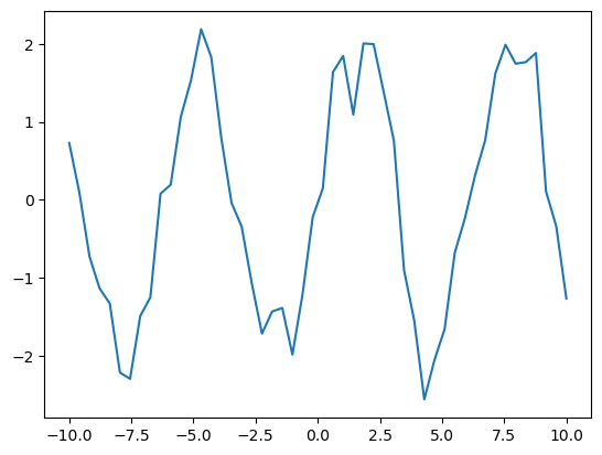
Say we observe some data $x_1, x_2, \dotsc$.

xs = torch.linspace(-10, 10, 50)

Assume there’s an unknown function $f$ that maps each data point $x_i$ to an unknown value $f_i$.

fs = 2*torch.sin(xs)

And each $f_i$ is associated with an observed noisy version $y_i$.

ys = fs + 0.4*torch.randn(xs.shape)

plt.plot(xs, ys);

Say we have some additional inputs $x_1^\ast, x_2^\ast, \dotsc$ and we want to estimate the associated $f^\ast_1, f^\ast_2, \dotsc$. We’ll assume that the $f_i$ and $f^\ast$, along with a latent vector $u$ of outouts at known inputs $z$, are all jointly Gaussian. The $u_i$ are known as inducing points. We’ll ensure that the conditional covariance structure is sparse, however: $f_i$ will be conditionally independent given $u$. This will keep the computation of the posterior tractable, even when we have a large number of training points $f$.

Specifically, say \(\begin{bmatrix} u \\ f \\ f^* \end{bmatrix} \sim \mathcal{N}\left(0, \begin{bmatrix} K_{uu} & K_{uf} & K_{u*} \\ K_{fu} & D_{ff} & K_{fu}K_{uu}^{-1}K_{u*} \\ K_{*u} & K_{*u}K_{uu}^{-1}K_{uf} & K_{**} \end{bmatrix} \right)\)

The expressions for conditionally independent covariances keep popping up, so We’ll abbreviate $K_{au}K_{uu}^{-1}K_{ub}$ as $Q_{ab}$. Using the standard Gaussian conditioning formula, we find that

\[\begin{bmatrix} f \\ f^* \end{bmatrix} \, \bigg \vert \, u \sim \mathcal{N} \left( \begin{bmatrix} K_{fu}K_{uu}^{-1}u \\ K_{*u}K_{uu}^{-1}u \end{bmatrix} , \begin{bmatrix} D_{ff} - Q_{ff} & Q_{f*} \\ Q_{*f} & K_{**} - Q_{**}\end{bmatrix} \right)\]

We’ll choose $D_{ff}$ so that $D_{ff} - Q_{ff}$ is diagonal. Specifically, we’ll let $D_{ff} = Q_{ff} + \text{Diag}(I - Q_{ff})$.

It remains to choose the dense covariances $K_{uu}$. We’ll choose a covariance structure that makes $u_i$ and $u_j$ close when $z_i$ and $z_j$ are.

def kernel(a,b):
    return torch.exp(-0.5*((a[:,None] - b[None,:])/2)**2)

z = torch.linspace(-8, 8, 10)

k_uu = kernel(z, z)
k_uu_chol = torch.linalg.cholesky(k_uu)
k_uu_inv = torch.cholesky_inverse(k_uu_chol)
k_fu = kernel(xs, z)
k_ff_given_u = torch.diag(torch.eye(fs.shape[0]) - (k_fu @ k_uu_inv @ k_fu.T)) + 1e-5
conditioner = k_fu @ k_uu_inv

This gives us a fully generative prior for the function values $f$ and inducing points $u$.

def model(obs):
    u = pyro.sample("u", dist.MultivariateNormal(torch.zeros(k_uu_inv.shape[0]), precision_matrix= k_uu_inv))
    with pyro.plate("data"):
        f = pyro.sample("f", dist.Normal(conditioner @ u, k_ff_given_u))
        return pyro.sample("obs", dist.Normal(f, 0.16), obs=obs) 

We’ll assume that the posterior over $u$ given our observations $y$ is Gaussian as well.

lower_cholesky = LowerCholeskyTransform()

def guide(obs):
    M = k_uu_inv.shape[0]
    m = pyro.param("m", torch.randn(M))
    S = lower_cholesky(pyro.param("S", k_uu_chol))
    return pyro.sample("u", dist.MultivariateNormal(m, scale_tril=S))

This guide only covers $u$, not $f$. The conditional distribution of $f$ given $u$ will be the same as in the prior because it’s independent of $y$. To let the model know that the associated guide has the same conditional distribution for $f$, we use Pyro’s block function. As $y$ here is Normally distributed about $f$, we could analytically marginalize out $f$. But we’ll keep things simple and use samples of $f$ instead.

marginalized_model = poutine.block(model, hide="f")

Training

We can fit the parameters in our variational approximation to maximize the ELBO using a standard Pyro training loop.

adam = pyro.optim.Adam({"lr": 0.03})
svi = SVI(marginalized_model, guide, adam, loss=Trace_ELBO())

pyro.clear_param_store()
for j in range(1500):
    loss = svi.step(ys)
    if j % 100 == 0:
        print(loss)

8269.271677017212
926.9810304641724
341.00060176849365
297.3144989013672
317.0104932785034
215.36338233947754
176.66253185272217
205.85192108154297
285.5180616378784
201.31714820861816
234.66797637939453
252.92035484313965
237.8198699951172
184.29428958892822
169.9394235610962

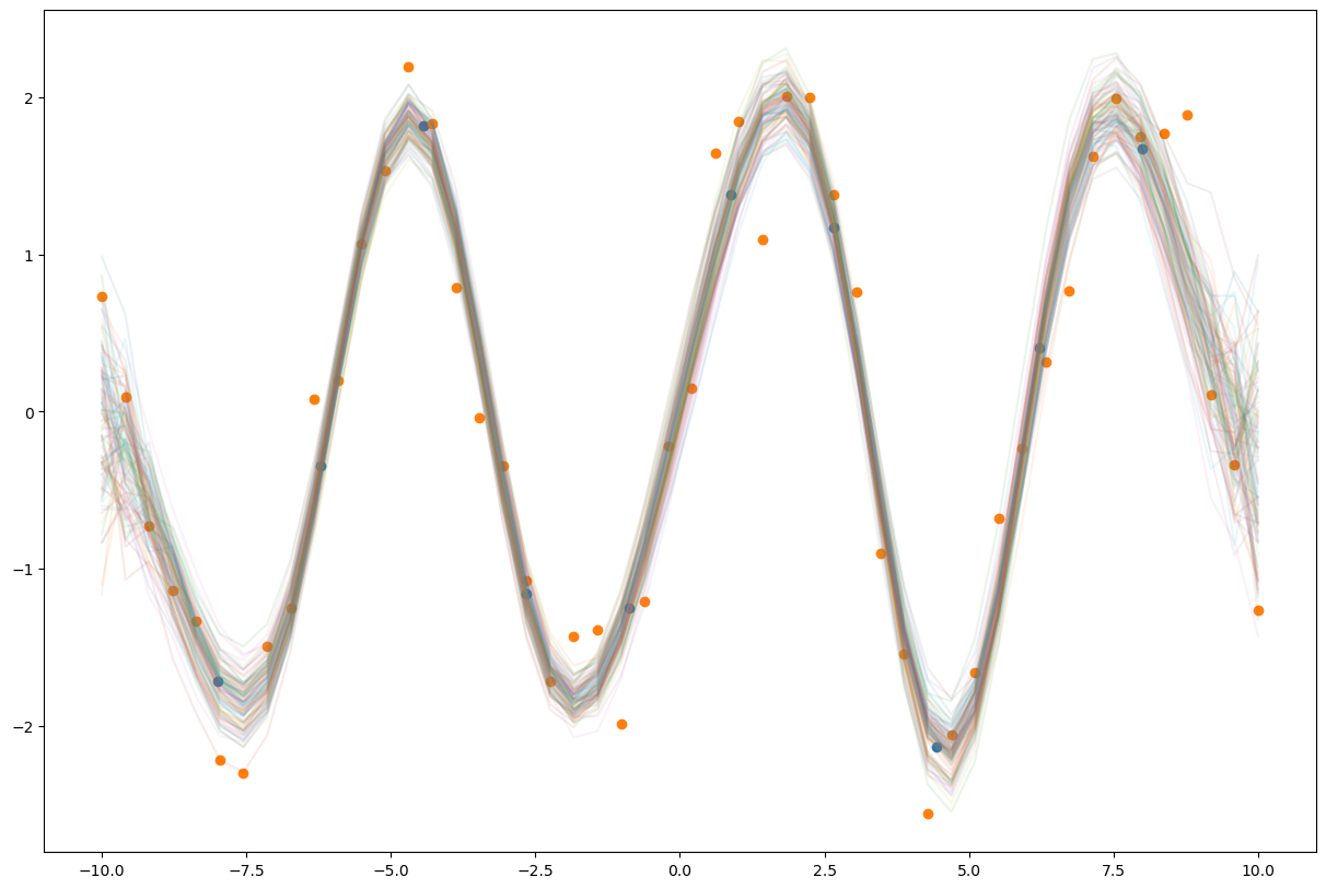
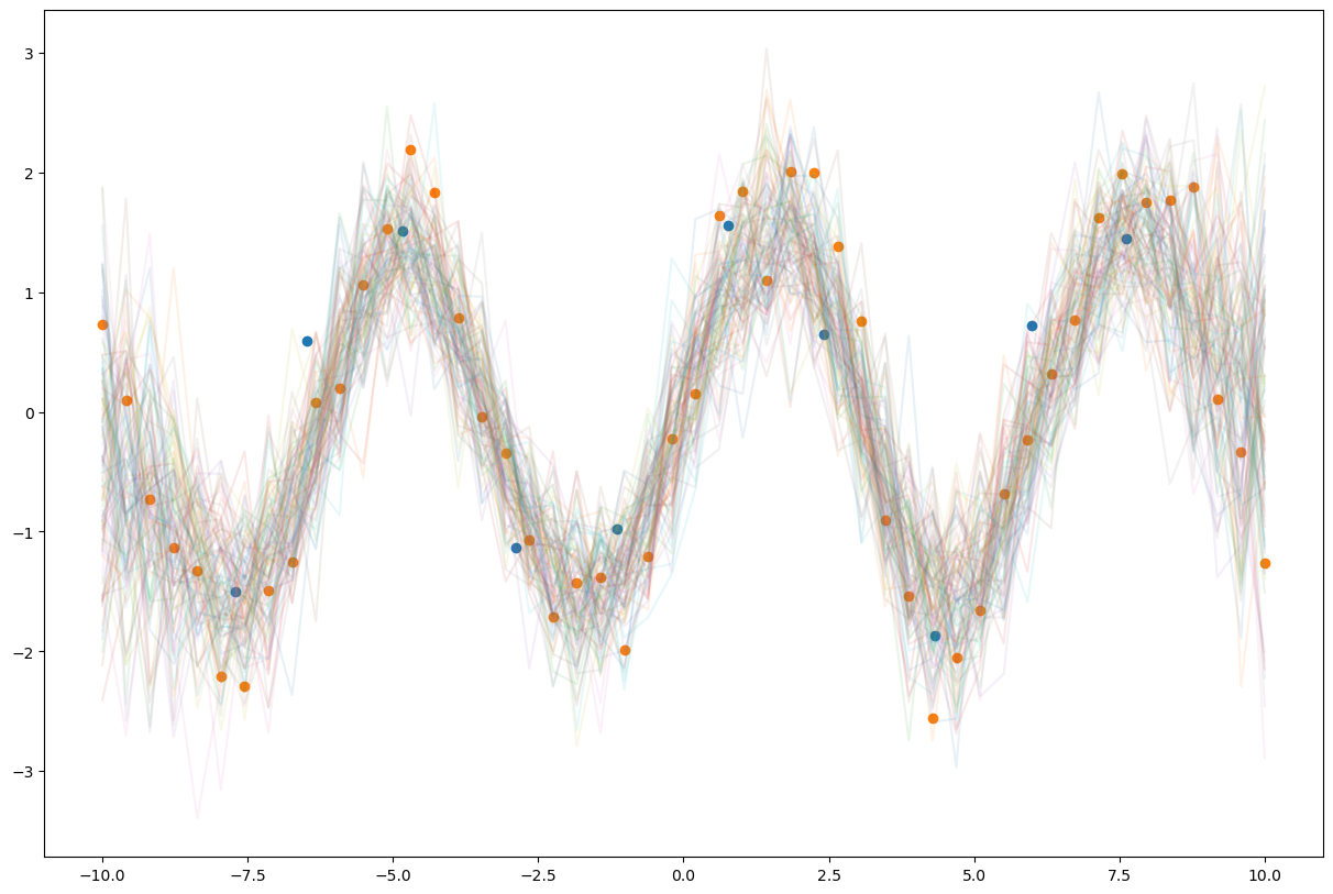
pred = Predictive(model, guide=guide, num_samples=100)

samples = pred(None)['f'].numpy()

plt.figure(figsize=(15,10))
plt.plot(xs, samples.T, alpha=0.1);
plt.scatter(z, pyro.param("m").detach().numpy())
plt.scatter(xs.numpy(), ys.numpy());

Using GPytorch

This approach to inference has is also available in pre-packaged from from the GPytorch library.

class GPModel(gp.models.ApproximateGP):
    def __init__(self, num_inducing=10):
        variational_strategy = gp.variational.VariationalStrategy(
            self, torch.linspace(-8, 8, num_inducing),
            gp.variational.CholeskyVariationalDistribution(num_inducing_points=num_inducing))
        super().__init__(variational_strategy)
        self.mean_module = gp.means.ConstantMean()
        self.covar_module = gp.kernels.ScaleKernel(gp.kernels.RBFKernel())
        
    def forward(self, x):
        mean = self.mean_module(x)
        covar = self.covar_module(x)
        return gp.distributions.MultivariateNormal(mean, covar)

gp_model = GPModel()

def guide(x, y):
    pyro.module("gp", gp_model)
    with pyro.plate("data"):
        pyro.sample("f", gp_model.pyro_guide(x))

def model(x, y):
    with pyro.plate("data"):
        f = pyro.sample("f", gp_model.pyro_model(x))
        return pyro.sample("obs", dist.Normal(f, 1.), obs=y) 

gp_model.train();

adam = pyro.optim.Adam({"lr": 0.03})
svi = SVI(model, guide, adam, loss=Trace_ELBO(retain_graph=True))

pyro.clear_param_store()
for j in range(1000):
    gp_model.zero_grad()
    loss = svi.step(xs, ys)
    if j % 100 == 0:
        print(loss)

108.06522274017334
70.28253173828125
71.7653317451477
70.8886947631836
72.2854871749878
77.09591293334961
66.6847620010376
71.59606075286865
63.947476387023926
79.98937606811523

gp_model.eval();

pred = Predictive(model, guide=guide, num_samples=100)

with torch.no_grad():
    samples = pred(xs, None)['f']

z = gp_model.variational_strategy.inducing_points.detach().numpy()
m = gp_model.variational_strategy._variational_distribution.variational_mean.detach().numpy()
plt.figure(figsize=(15,10))
plt.plot(xs.numpy(), samples.T.numpy(), alpha=0.1)
plt.scatter(z, m)
plt.scatter(xs.numpy(), ys.numpy())

<matplotlib.collections.PathCollection at 0x7fbb1d882790>

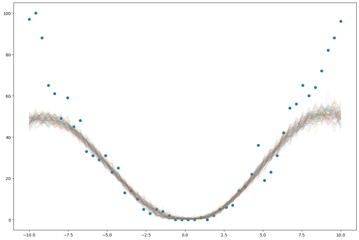
Using a non-Gaussian Likelihood

We don’t always need $y$ to be a version of $f$ with added noise. We can use an arbitrary stochastic function of $f$. For example, say we observe discrete count data instead. We’d like our likelihood to be Poisson.

gp_model = GPModel()

def model(x, y):
    with pyro.plate("data"):
        f = pyro.sample("f", gp_model.pyro_model(x))
        return pyro.sample("obs", dist.Poisson(F.softplus(f)), obs=y) 

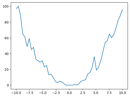
latent_fs = xs**2

ys = dist.Poisson(latent_fs).sample()

plt.plot(xs, latent_fs)

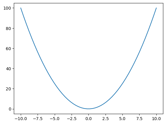
plt.plot(xs, ys)

gp_model.train();

adam = pyro.optim.Adam({"lr": 0.03})
svi = SVI(model, guide, adam, loss=Trace_ELBO(retain_graph=True))

pyro.clear_param_store()
for j in range(1000):
    gp_model.zero_grad()
    loss = svi.step(xs, ys)
    if j % 100 == 0:
        print(loss)

5798.9597454071045
1725.3109169006348
924.9359188079834
664.2655711174011
546.4507675170898
516.206377029419
475.42826652526855
491.79768562316895
444.60411643981934
447.5388412475586

gp_model.eval();

pred = Predictive(model, guide=guide, num_samples=100)

with torch.no_grad():
    samples = pred(xs, None)['f']

plt.figure(figsize=(15,10))
plt.plot(xs, F.softplus(samples.T).numpy(), alpha=0.1)
plt.scatter(xs, ys)