In a \(k\)-Nearest Neighbor Gaussian Process, we assume that the input points \(x\) are ordered in such a way that \(f(x_i)\) is independent of \(f(x_j)\) whenever \(i > j + k\). When \(k=2\), for example, this means we can generate the sequence of process values by sampling the first value, then sampling the second given the first, then the third given the first two, then the fourth given the second and third, and so on.
The conditional distribution for \(f_i\) with \(k\)-predecessors in the set \(S\) has mean \(K_{i, S}K_{S,S}^{-1} f_S\) and variance \(K_{i, i} - K_{i, S}K_{S,S}^{-1} K_{i,S}\). This means we can write the generation procedure as
where \(\eta_i \sim \mathcal{N}(0, K_{i, i} - K_{i, S}K_{S,S}^{-1} K_{i,S})\). In matrix form, this means
where \(B\) is the strictly lower triangular matrix that comes from stacking zero-padded rows of the form \(K_{i, S}K_{SS}^{-1}\). This shows that \(f\) has a precision matrix of the form \(UU^T\) where \(L=(I - B)^TF^{-1/2}\) and \(F\) is diagonal.
Implementation
using KernelFunctions, LinearAlgebra, SparseArrays, AbstractGPs
We assume that pts are in order, and that each point is independent of all the previous ones given the previous k.
function make_B(pts::AbstractVector{T}, k::Int, kern::Kernel) where {T}
    n = length(pts)
    js = Int[]
    is = Int[]
    vals = T[]
    for i in 1:n
        if i == 1
            ns = T[]
        else
            ns = pts[max(1, i - k):i-1]
        end
        row = kernelmatrix(kern, ns) \ kern.(ns, pts[i])
        start_ix = max(i - k, 1)
        col_ixs = start_ix:(start_ix+length(row)-1)
        append!(js, col_ixs)
        append!(is, fill(i, length(col_ixs)))
        append!(vals, row)
    end
    sparse(is, js, vals, n, n)
end;
To the understand the form of the B matrix described above more clearly, consider its form in a 2-nearest neighbor Gaussian Process.
pts = [1.0, 2.0, 3.5, 4.2, 5.9, 8.0];
kern = SqExponentialKernel();
B = make_B(pts, 2, kern)
6×6 SparseMatrixCSC{Float64, Int64} with 9 stored entries:
   ⋅          ⋅          ⋅          ⋅          ⋅         ⋅
  0.606531    ⋅          ⋅          ⋅          ⋅         ⋅
 -0.242002   0.471434    ⋅          ⋅          ⋅         ⋅
   ⋅        -0.184647   0.842651    ⋅          ⋅         ⋅
   ⋅          ⋅        -0.331424   0.495153    ⋅         ⋅
   ⋅          ⋅          ⋅        -0.0267458  0.116556   ⋅
The \(F\) matrix can be constructed analogously.
function make_F(pts::AbstractVector{T}, k::Int, kern::Kernel) where {T}
    n = length(pts)
    vals = T[]
    for i in 1:n
        prior = kern(pts[i], pts[i])
        if i == 1
            push!(vals, prior)
        else
            ns = pts[max(1, i - k):i-1]
            ki = kern.(ns, pts[i])
            push!(vals, prior - dot(ki, kernelmatrix(kern, ns) \ ki))
        end
    end
    Diagonal(vals)
end;
F = make_F(pts, 2, kern)
6×6 Diagonal{Float64, Vector{Float64}}:
 1.0   ⋅         ⋅         ⋅         ⋅         ⋅
  ⋅   0.632121   ⋅         ⋅         ⋅         ⋅
  ⋅    ⋅        0.857581   ⋅         ⋅         ⋅
  ⋅    ⋅         ⋅        0.356873   ⋅         ⋅
  ⋅    ⋅         ⋅         ⋅        0.901874   ⋅
  ⋅    ⋅         ⋅         ⋅         ⋅        0.987169
The associated covariance matrix has the form \((I-B)^{-1}F(I-B)^{-1}\). We can compare this approximation to the full (non nearest-neighbor) covariance matrix.
L = (I - B) \ sqrt(F)
6×6 Matrix{Float64}:
  1.0          0.0          0.0        0.0        0.0      0.0
  0.606531     0.79506      0.0        0.0        0.0      0.0
  0.0439369    0.374819     0.926056   0.0        0.0      0.0
 -0.0749706    0.169036     0.780342   0.597388   0.0      0.0
 -0.0516836   -0.0405252    0.0794716  0.295798   0.94967  0.0
 -0.00401888  -0.00924444  -0.011608   0.0184994  0.11069  0.993564
L * L'
6×6 Matrix{Float64}:
  1.0          0.606531     0.0439369  -0.0749706    -0.0516836  -0.00401888
  0.606531     1.0          0.324652    0.0889216    -0.0635677  -0.00978746
  0.0439369    0.324652     1.0         0.782705      0.0561348  -0.0143912
 -0.0749706    0.0889216    0.782705    1.0           0.235746    0.000731802
 -0.0516836   -0.0635677    0.0561348   0.235746      1.0         0.110251
 -0.00401888  -0.00978746  -0.0143912   0.000731802   0.110251    1.0
kernelmatrix(kern, pts)
6×6 Matrix{Float64}:
 1.0          0.606531     0.0439369   0.00597602   6.11357e-6   2.28973e-11
 0.606531     1.0          0.324652    0.0889216    0.000497955  1.523e-8
 0.0439369    0.324652     1.0         0.782705     0.0561348    4.00653e-5
 0.00597602   0.0889216    0.782705    1.0          0.235746     0.000731802
 6.11357e-6   0.000497955  0.0561348   0.235746     1.0          0.110251
 2.28973e-11  1.523e-8     4.00653e-5  0.000731802  0.110251     1.0
The two are pretty close!
Interface
To make this usable with Julia's AbstractGPs library, we'll add a new method for the posterior function.
struct NearestNeighbors
    k::Int
end
struct InvRoot{A}
    U::A
end
AbstractGPs.diag_Xt_invA_X(A::InvRoot, X::AbstractVecOrMat) = AbstractGPs.diag_At_A(A.U' * X)
function AbstractGPs.posterior(nn::NearestNeighbors, fx::AbstractGPs.FiniteGP, y::AbstractVector)
    kern = fx.f.kernel
    F = make_F(fx.x, nn.k, kern)
    B = make_B(fx.x, nn.k, kern)
    U = UpperTriangular((I - B)' * inv(sqrt(F)))
    δ = y - mean(fx)
    α = U * (U' * δ)
    C = InvRoot(U)
    AbstractGPs.PosteriorGP(fx.f, (α=α, C=C, x=fx.x, δ=δ))
end
Here's how we use it:
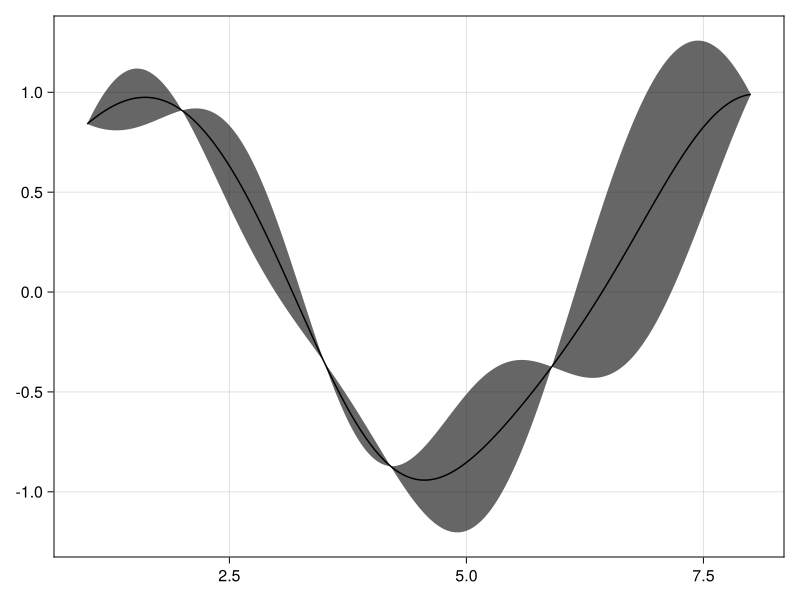
y = sin.(pts);
fx = GP(kern)(pts, 0.0);
Note that the nearest neighbor approximation requires a noise-free GP.
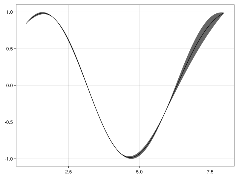
post = posterior(NearestNeighbors(5), fx, y);
using CairoMakie, AbstractGPsMakie
plot(1:0.01:8, post)
Optimizing Hyperparameters
The last thing necessary to make this technique usable in practice is to ensure it works with autodifferentiation so that we can optimize hyperparameters like lengthscales.
using ForwardDiff, ParameterHandling, Optim, Zygote
initial_params = (var=positive(1.0), lengthscale=positive(1.0));
flat_initial_params, unflatten = ParameterHandling.value_flatten(initial_params);
function build_gp(params)
    k2 = params.var * with_lengthscale(kern, params.lengthscale)
    GP(k2)(pts, 0.0)
end;
function objective(flat_params)
    params = unflatten(flat_params)
    fx = build_gp(params)
    -logpdf(fx, y)
end;
training_results = Optim.optimize(
    objective,
    θ -> only(Zygote.gradient(objective, θ)),
    flat_initial_params,
    BFGS(
        alphaguess=Optim.LineSearches.InitialStatic(scaled=true),
        linesearch=Optim.LineSearches.BackTracking(),
    ),
    inplace=false,
)
 * Status: success

 * Candidate solution
    Final objective value:     4.130829e+00

 * Found with
    Algorithm:     BFGS

 * Convergence measures
    |x - x'|               = 2.86e-07 ≰ 0.0e+00
    |x - x'|/|x'|          = 4.80e-07 ≰ 0.0e+00
    |f(x) - f(x')|         = 2.06e-12 ≰ 0.0e+00
    |f(x) - f(x')|/|f(x')| = 4.98e-13 ≰ 0.0e+00
    |g(x)|                 = 4.43e-09 ≤ 1.0e-08

 * Work counters
    Seconds run:   0  (vs limit Inf)
    Iterations:    11
    f(x) calls:    18
    ∇f(x) calls:   12
With optimized parameters, we get much less uncertainty in our predictions.
plot(1:0.01:8, posterior(NearestNeighbors(5),
    build_gp(unflatten(training_results.minimizer)), y))